Graph Simplfication for a Faster A*

A* is an algorithm that is so well covered that I won’t be wasting my time to add to the noise in this blog post, but if you are unfamiliar with A*, I recommend reading an introduction from Red Blob Games and then coming back here.¹

Alright, assuming you are familiar with A*, the question you may be having is: “How can we make A* faster?” There are, in fact, a lot of ways. If you don’t care about finding an optimal path, you can use an inadmissable heuristic.² If you wish to reduce resources required, you can cache common path requests. If you have a problem where the path is constantly being recalculated, then you can migrate to D*. If you want every search possible to be less costly to compute while still being optimal, you have to do something different. Specifically, you need to reduce the search space.³

Because this is a blog post, I am not going to cover all the related work. In fact, I made the mistake of not doing any searching beforehand when I came up with this method. From what I can tell now, after the fact, this method is not new or particularly innovative. It is, though, in my opinion, cool. The way it works is by taking a graph and simplifying it by turning it into a graph of graphs. Then, A* runs on the top level graph, before going into the subgraph. The result, as we’ll see, is a faster A*. The cost, though, is that you have to run graph simplification offline. If you have a graph that is constantly changing, this is not the method for you.

The rest of this post is broken into sections. In the first, I show how mazes are generated. In the second, I describe the algorithm for simplifying grpahs. In the third, I show the results and discuss them. The final section discusses the limitations and areas for improvement.

Generating Mazes

The code below is for generating a maze which is represented as a graph. For the graph, NetworkX is used. A grid_graph is used to create the graph. Then the weight of every edge in the graph is set randomly. This makes it so each maze generated is different when the minimum spanning tree is created. The default algorithm used by NetworkX is Kruskal’s Algorithm.⁴

import networkx as nx
from random import random

def generate_maze(grid_size: int) -> nx.Graph:
    G = nx.grid_graph((grid_size, grid_size))

    for u,v in G.edges:
        G.edges[(u,v)]['weight'] = random()

    return nx.minimum_spanning_tree(G)

Simplifying Graphs

The method I came up with—I am not saying that I am the first to have this idea—is that a graph can be simplified by looking for critical nodes and condensing the rest down to a subgraph. A critical node is any node that has a degree of greater than two. A node’s degree is determined by the number of incoming and outgoing edges.

The code (see below) starts by finding all such critical nodes, and intializing a node_lookup dictionary. The dictionary is not required, but it is useful. Take a simple example where we want to find a path fron node A to node C. In a regular graph, we could look up both by name in an 0(1) operation and everything is hunkydory. If, though, either A or C are in a sub-graph, we’re in trouble. We’ll have to look through every node until we find what we’re looking for. The node_lookup dictionary address this by allowing us to again have an 0(1) operation.

Now, onto the actual algorithm. It starts by looping through every critical node and updating the lookup table. The next step is to loop through the edges that are connected to the critical node. For each of these, it follows the edges until another critical node is found. Then, every non-critical node found is condensed into one sub-graph. The subgraph replaces the original set of uncritical nodes. Then an edge from the original node to the subraph is made, and an edge from the subraph to the newly found critical node is added if a critical node was found—if a critical node was not found, then no outgoing edge is added because the last node was a leaf. Finally, the node lookup table is updated, and that is it. A pretty simple algorithm, at least I think.

def build_hyper_graph(G: nx.Graph) ->  Dict[str, str]:
    critical_nodes = [n for n in G.nodes() if G.degree(n) > 2]
    node_lookup = {}

    for n in critical_nodes:
        node_lookup[n] = n
        next_nodes = list(G.edges(n))

        for _, a_2 in next_nodes:
            if a_2 in critical_nodes:
                continue

            if not G.has_edge(n, a_2):
                continue

            G.remove_edge(n, a_2)
            weight = 0
            nodes = [a_2]
            a_1 = n
            a_3 = None
            while True:
                if a_2 in critical_nodes:
                    nodes.pop()
                    break

                edges = G.edges(a_2)
                if len(edges) == 0:
                    G.remove_node(a_2)
                    a_1 = None
                    break

                for _, a_3 in G.edges(a_2):
                    if a_1 != a_3:
                        break

                weight += G.edges[(a_2, a_3)][W]
                nodes.append(a_3)
                G.remove_edge(a_2, a_3)
                G.remove_node(a_2)

                a_1 = a_2
                a_2 = a_3

            hyper_state_name = '||'.join(str(node_name) for node_name in nodes)
            for node_name in nodes:
                node_lookup[node_name] = hyper_state_name

            critical_nodes.append(hyper_state_name)
            G.add_edge(n, hyper_state_name, weight=weight, color='BLACK')

            if a_1 != None:
                G.add_edge(hyper_state_name, a_3, weight=0, color='BLACK')

    return node_lookup

Results

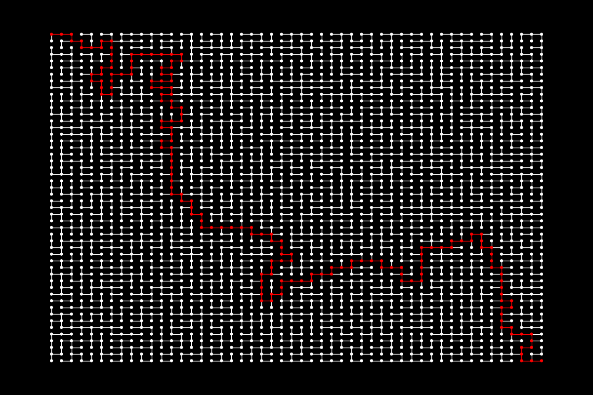Original maze	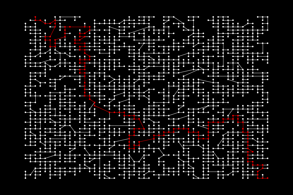Simplified maze

In the first figure above, you can see a simple example of what happens when we take a big maze where the red line marks the solution, and we simplify it and run A* again. Just from a visual, it can be seen that the search space is reduced. But, by how much?

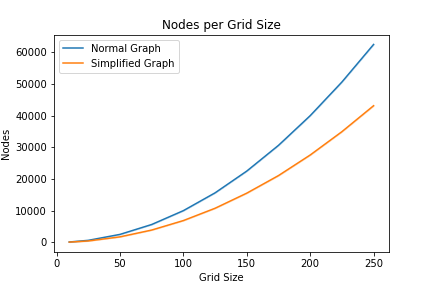Reduction for nodes.	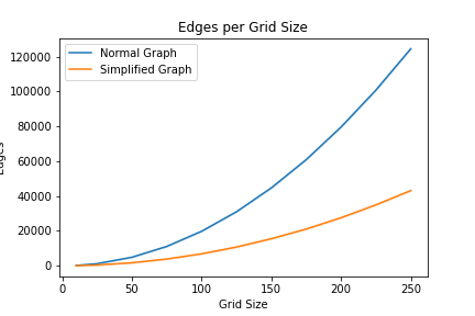Reduction for edges.

As you can see, the larger the graph becomes, the more signifigant the reduction in nodes and edges.⁵ More specifically, this results in an overall number of nodes reduced by ~31.4% and edges by ~65.1%. But, how much does this affect the overall speed of A*?

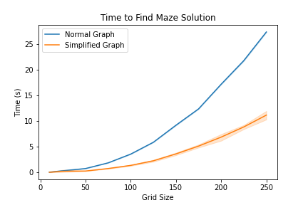A* solution time.

We again find similar results where the larger the graph becomes, the more significant the overall reduction in time spent running A*.

Limitations and Areas for Improvement

• The method should be tested with multiple pathfinding tasks rather than just mazes. For example, it would be interesting to see how it performed on a graph of city streets for a city like Chicago or New York.
• The timing benchmark was run locally and not on a server, it used an imprecise clock, and did not do many of the things one should do when trying to say “X is faster than Y.”
• The example only runs with one subraph, but it could be even faster if more layers were built. The build_hyper_graph function could be recursive and call itself until only critical nodes were in the top-level graph.
• No work was done to evaluate at what graph size this method becomes fast enough to be worthwhile. It can be examined visually from the plot above to be around 100x100, or ten-thousand nodes, but result may vary given different graph structures.
• The problem evaluated for timing was to find a path from the top-left node to the bottom-right node. A more thorough approach would have been to test pathfinding between all nodes.
• The method works for an undirected graph, but has not been tested or shown to work with a digraph.

There are more limitations and areas for improvement, but those are the major ones that come to mind. I hope that you enjoyed this post, and feel free to reach out if you have any questions.⁶