In this set of posts, I want to go over Q-learning (a form of reinforcement learning). To start, we could go in two directions. We could explore at the bottom and look at the math behind neural networks and Q-learning. Or we could start at the top and see the end result. We are going to go with the latter.

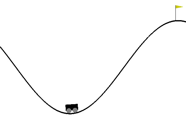
Figure 1: the mountain car environment.

To do this we are going to need a few libraries and a testbed. To test, we are going to use OpenAI’s Gym and use MountainCar-V0. In this environment, proposed by Andrew Moore in his Ph.D. thesis, the car must reach the flag seen in figure 1. The car, though, does not have enough acceleration to achieve this by just going forward. Instead, it must go back and forward, steadily gaining enough speed to reach the goal. This is a problem that can be solved simply with a rule-based agent, however, reinforcement approaches can struggle with this. You’ll soon see that the amount of episodes it takes for q-learning to solve this is more than expected.

We are going to need to install gym, keras, and keras-rl. All of these can be installed with pip install X. I would recommend using anaconda when possible. Keras is a library built to use TensorFlow, CNTK, or Theano. Each of these three are neural network libraries that we can use to define networks. Keras makes it easy to use any of these and provides a very intuitive way to define networks. Also, when installing Keras it may be configured to use a library for neural networks you do not want to use; if you encounter this issue, please visit this site. Keras-RL is a reinforcement learning library built on top of Keras which allows us to run reinforcement algorithms on Keras networks for any gym environment. Meaning, the code is incredibly simple for this post. As a note, TensorFlow does provide Keras built in, but this will not work with Keras-RL. You need to use Keras for this stage.

With that done, we can start building our example without having a clue about anything we’re doing. As a side note, I don’t know if this is necessarily a good thing because it allows people access to technology that can be used very unethically. Though in this case, we are using it to learn the basics and gather an intuition for Q-learning. The first thing we need to do is to create our learning environment:

import gym
env = gym.make('MountainCar-v0')

We can now define our network:

from keras.models import Sequential
from keras.layers import Dense, Activation, Flatten
from keras.optimizers import Adam

model = Sequential()
model.add(Flatten(input_shape=(1,) + env.observation_space.shape))
model.add(Dense(128))
model.add(Activation('relu'))
model.add(Dense(64))
model.add(Activation('relu'))
model.add(Dense(32))
model.add(Activation('relu'))
model.add(Dense(env.action_space.n))
model.add(Activation('linear'))

First, notice that the first layer of the model is based on the observation space of the environment. This is telling the neural network what kind of input it should be expecting. At the tail end, you have a a layer that has the size of the action space. This means that for every action possible, the network will have an output node. Each output node represents an action that can be taken and the node with the highest output value will be used as an action for the given step. The rest of the network has important details that we are going to ignore. We only want to cover the basics and we will come back as we leave the top view and approach the bottom.

Now that we have a network and an environment, we need it to learn. Better put, we need to have our network play a bunch of games and update itself to play even better. To do this, as mentioned, we are going to use Q-learning that has been implemented in Keras-RL.

from rl.memory import SequentialMemory
from rl.policy import BoltzmannQPolicy
from rl.agents import DQNAgent

dqn = DQNAgent(
    model=model, 
    nb_actions=env.action_space.n, 
    memory=SequentialMemory(limit=50000, window_length=1), 
    nb_steps_warmup=10,
    target_model_update=1e-2, 
    policy=BoltzmannQPolicy())

dqn.compile(Adam(lr=1e-3), metrics=['mae'])
dqn.fit(env, nb_steps=150000, visualize=False, verbose=2)
dqn.save_weights('model.mdl', overwrite=True)
dqn.test(env, nb_episodes=5, visualize=True)

In this block of code, there is a lot of things that, likely, will not make sense. For example, what is the BoltzmanQPolicy? At the moment, it is isn’t important so treat it like a black box. What is important in this block of code is that we can see the agent runs for 150,000 steps. Each game is composed of 200 steps which mean we give the agent 750 games to learn how to play the game. In my brief experiments with how many steps were necessary, this seemed to be the right amount. You’ll also notice that we have visualize while training set to false. This makes it so gym does not render every game which saves compute and will speed up our training time. After training, we save the model and run a test to see how it works.

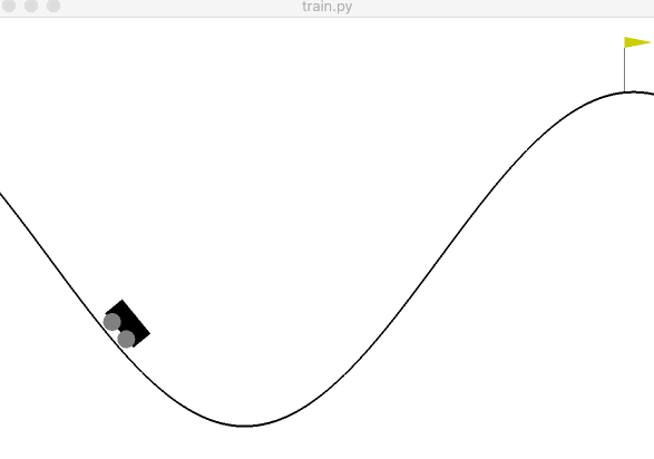
Figure 2: an example of the agent successfully reaching the target.

If all went well, you’ll have a result similar to figure 2. The source code of this project can be found on GitHub. You’ll notice I added command line arguments and some functions to make the code cleaner and easier to use when experimenting. In the next post, we are going to peel back the first layer and look into q-learning. We will either implement it and then go over the theory or do the opposite. I’m not sure yet which is best yet, so I’m not committing to either. In the meantime, I’d recommend playing with the variables to gain an intuition for reinforcement learning. Try to get a feel for why the agents in bigger examples like OpenAI’s Dota 2 bot or DeepMind’s AlphaZero required so many computers to learn how to play these more complicated games.

Citation